
Documentation
This guide walks through the core sftools interfaces, from state containers and models to estimation and plotting.
For installation and a first example, start with Getting started.
Contents
- Dimension conventions
- State containers
- Dynamic models
- Observation models
- Least-squares estimation
- Recursive filtering
- Moment transforms
- Analysis and plotting
- API quick reference
- Example manual (PDF)
Dimension conventions
Model calculations represent states, observations, and sample collections as columns.
| Quantity | Shape |
|---|---|
| One state | (n, 1) |
| One observation | (m, 1) |
| State or sample collection | (n, N) |
| Predicted observations for a collection | (m, N) |
| Measurement Jacobian at one state | (m, n) |
| Measurement covariance | (m, m) |
ls, wls, nls, helper.llh, and filter measurement updates require a single observation in column form.
They reject flat, row, and batched observations rather than silently reshaping them or allowing accidental broadcasting.
Convert a flat observation explicitly with y[:, None].
Each particle-filter update applies one observation to all particles.
GaussianState.x stores its mean as a flat (n,) array; state.mean() returns it as an (n, 1) column.
Built-in models also accept flat state inputs, while custom model callbacks must return the expected shapes.
nls handles SciPy’s flat optimization-vector convention internally.
State containers
Import shared containers from the package root or sftools.types:
import numpy as np

from sftools import GaussianState, ParticleState, StateTrajectory

state = GaussianState(x=np.array([1.0, 2.0]), P=np.diag([0.5, 0.2]))
print(state.mean())  # (2, 1)
print(state.cov())   # (2, 2)

rng = np.random.default_rng(0)
particles = rng.multivariate_normal(state.x, state.P, size=500).T
particle_state = ParticleState(particles, np.full(500, -np.log(500)))

trajectory = StateTrajectory.preallocate(state_dim=2, steps=5, with_cov=True)
for k in range(5):
    trajectory.write_state(k, GaussianState(state.x + k, state.P))
ParticleState stores particles as (n, N) columns and log weights as (N,).
Its .mean() and .cov() compute weighted empirical moments.
Use write_state to record estimates and covariances, or write_mean for deterministic trajectories.
Iteration over a StateTrajectory yields (n, 1) state columns.
trajectory.component(0) selects a component across time.
trajectory.iter_samples(include_cov=True, include_time=True) yields (y, cov, t) tuples when those data are available.
Dynamic models
Create a model with sftools.create_dynamics(name, ...).
Each dynamic model provides f(x) for deterministic propagation, F(x) for its Jacobian, G(x) for process-noise gain, and random(n=1, x=None, rng=None) for stochastic propagation.
| Name | State layout | Constructor arguments |
|---|---|---|
linear |
User-defined | F, G, Q |
cv |
Positions followed by velocities, 2n states |
T, Q, n |
ct |
[x, y, speed, heading, turn_rate] |
T, Q, n (n unused) |
import numpy as np
from sftools import create_dynamics

dyn = create_dynamics("cv", T=0.1, Q=0.01 * np.eye(2), n=2)
x = np.array([[0.0], [0.0], [1.0], [0.5]])
predicted = dyn.f(x)
jacobian = dyn.F(x)
samples = dyn.random(n=3, x=x, rng=np.random.default_rng(1))
T is the sampling interval, and Q is the process-noise covariance.
Match T to your data and ensure the dimensions of Q match the model.
Observation models
Create an observation model with sftools.create_observation(name, ...).
Each model provides h(x) for expected measurements, H(x) for the Jacobian at one state, and random(x, n=1, rng=None) for noisy observations.
Its measurement covariance is available as model.R.
| Name | Measurement | Constructor arguments |
|---|---|---|
linear |
Linear mapping H @ x |
H, R |
nonlinear |
User-supplied mapping and Jacobian | h, H, R, **kwargs |
pos |
Direct position observation | R, n |
toa |
Range to each anchor | p, R, n |
tdoa |
Range differences relative to the first anchor | p, R, n |
tdoa_r0 |
Range with an unknown common offset | p, R, n |
Anchor positions are columns of p:
import numpy as np
from sftools import create_observation

anchors = np.array([[0.0, 10.0, 10.0, 0.0], [0.0, 0.0, 10.0, 10.0]])
obs = create_observation("toa", p=anchors, R=0.01 * np.eye(4), n=4)
x = np.array([[3.0], [4.0]])
expected = obs.h(x)
jacobian = obs.H(x)
measurement = obs.random(x=x, rng=np.random.default_rng(2))
For custom nonlinear models, h must accept state collections of shape (n, N) and return measurements of shape (m, N).
H evaluates one state and returns a Jacobian of shape (m, n).
Range-model Jacobians are undefined at sensor positions; choose linearization and optimization starting points away from anchors.
Least-squares estimation
The static estimators are in sftools.estimator:
| Function | Purpose |
|---|---|
ls(model, y, x0) |
Unweighted least squares, locally linearized at x0 |
wls(model, y, x0) |
Covariance-weighted least squares, locally linearized at x0 |
nls(model, y, x0) |
Iterative nonlinear least squares |
All three return a GaussianState by default.
ls requires a full-column-rank design matrix and reports covariance A @ R @ A.T, where A is the unweighted least-squares gain.
With unequal or correlated measurement noise, it generally differs from the covariance returned by wls.
For range localization using the observation model above:
import matplotlib.pyplot as plt
from sftools import estimator, plot

initial_guess = np.array([[5.0], [5.0]])
estimate = estimator.nls(obs, measurement, initial_guess)
print(estimate.mean(), estimate.cov())

fig, ax = plt.subplots()
ax.plot(x[0, 0], x[1, 0], "o", label="True position")
plot.estimate(estimate, conf=0.95, label="NLS estimate", ax=ax)
ax.set_xlabel("Position x")
ax.set_ylabel("Position y")
ax.set_aspect("equal")
ax.legend(loc="lower center", bbox_to_anchor=(0.5, 1.02), ncol=2)
plt.show()
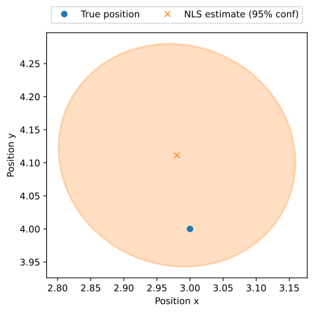
The plot zooms in on the estimated position; the four anchors are outside the displayed area. The ellipse shows the estimate’s local covariance.
nls uses Levenberg-Marquardt with the model’s analytic Jacobian and measurement covariance.
Request return_result=True to inspect termination and residuals.
Convergence alone does not establish global optimality or identifiability.
To retain the optimizer diagnostics, request the frozen NLSResult container:
from sftools import estimator

fit = estimator.nls(model, y, x0, return_result=True)
print(fit.optimizer.success, fit.optimizer.message)
print("Weighted residual sum of squares:", 2 * fit.optimizer.cost)
if fit.estimate is not None:
    print(fit.estimate.mean(), fit.estimate.P)
fit.optimizer is SciPy’s original OptimizeResult; its fun contains the
whitened residuals and jac their Jacobian. Nonconvergence raises
RuntimeError, and singular local covariance raises
numpy.linalg.LinAlgError when returning the ordinary estimate. With
return_result=True, either case returns estimate=None while preserving the
optimizer result. Successful termination does not establish global optimality,
identifiability, or confidence-region coverage.
Recursive filtering
KalmanFilter implements extended Kalman filtering, reducing to a standard Kalman filter for linear models.
UnscentedKalmanFilter uses sigma-point propagation.
ParticleFilter implements bootstrap particle filtering.
Filters expose meas_update(state, obs_model, y) and time_update(state).
There is deliberately no single filter(...) call that runs the whole recursion: you write the loop yourself and call the two updates explicitly.
This has two purposes:
- Understanding the two-stroke filtering engine. Every recursive filter alternates a measurement update (incorporate the observation) and a time update (predict to the next step). Writing the loop makes this structure visible and the same for all three filters.
- Flexible, accessible outlier rejection. Because you control the loop, you can inspect each observation (for example its innovation or a gating test) and skip
meas_updatefor outliers, or treat them differently, using ordinary Python and no special filter options.
The example below updates the prior with each observation, records the posterior, then predicts the state for the next time step:
import numpy as np

from sftools import GaussianState, StateTrajectory, create_dynamics, create_observation
from sftools import estimator

rng = np.random.default_rng(4)
steps = 40
dyn = create_dynamics("cv", T=0.1, Q=0.05 * np.eye(2), n=2)
obs = create_observation("pos", R=0.4 * np.eye(2), n=2)
filt = estimator.KalmanFilter(dyn_model=dyn)

truth = StateTrajectory.preallocate(state_dim=4, steps=steps, with_cov=False)
estimates = StateTrajectory.preallocate(state_dim=4, steps=steps, with_cov=True)
x = np.array([[0.0], [0.0], [1.0], [0.3]])
state = GaussianState(x=np.zeros(4), P=8.0 * np.eye(4))

for k in range(steps):
    truth.write_mean(k, x.ravel())
    y = obs.random(x=x, rng=rng)
    state = filt.meas_update(state, obs, y)
    estimates.write_state(k, state)
    state = filt.time_update(state)
    x = dyn.random(x=x, rng=rng)

rmse = np.sqrt(np.mean((estimates.mean[:2] - truth.mean[:2]) ** 2))
print(f"Position RMSE: {rmse:.3f}")
Output:
Position RMSE: 0.300
Initialize a particle filter from a Gaussian prior with init_state_gaussian(mean, cov, n_particles); it uses the filter’s random generator.
Tune process noise, measurement noise, and initial covariance with reproducible synthetic cases before using real data.
Inspect innovations and uncertainty—a plausible trajectory can still be overconfident.
Moment transforms
sftools.helper propagates state moments through nonlinear mappings:
| Function | Method |
|---|---|
ut(state, fun, ...) |
Unscented transform |
tt(state, fun) |
Taylor transform with supplied derivatives |
mct(state, fun, n_samples=..., rng=...) |
Monte Carlo transform |
Each returns a GaussianState by default.
For tt, pass fun=(f, F) for first-order propagation or fun=(f, F, H) to include second-order terms. Here, F is the Jacobian and H contains the output Hessians.
For example, transform polar coordinates to Cartesian coordinates:
import numpy as np
from sftools import GaussianState, helper

def polar_to_cartesian(x):
    r, theta = x[0], x[1]
    return np.stack((r * np.cos(theta), r * np.sin(theta)), axis=0)

polar = GaussianState(np.array([10.0, 0.2]), np.diag([0.5**2, 0.05**2]))
ut_estimate = helper.ut(polar, polar_to_cartesian)
mc_estimate = helper.mct(
    polar, polar_to_cartesian, n_samples=20_000, rng=np.random.default_rng(3)
)
Monte Carlo callbacks must return (n_outputs, n_samples), or (n_samples,) for scalar outputs.
At least two samples are required.
Covariance is always a matrix, including (1, 1) for a scalar output.
helper.sigma_points(state, alpha=..., beta=..., kappa=...) returns the points,
mean weights, and covariance weights used by the unscented transform. For an
n-dimensional input, the point array has shape (n, 2*n+1) and each weight
array has shape (2*n+1,). The first point is the mean, followed by positive
and negative Cholesky-column offsets. Mean and covariance weights are separate;
covariance weights need not sum to one and can be negative.
helper.ut returns a GaussianState by default. Its
return_sigma_points=True option returns the estimate, input points, and
output points. To retain Monte Carlo samples, call
helper.mct(..., return_result=True). The returned MCTResult keeps the
samples used for the estimate, so requesting them adds no random draws or
callback evaluations. Input and output samples have shapes
(n_inputs, n_samples) and (n_outputs, n_samples); scalar outputs have shape
(1, n_samples). Monte Carlo covariance uses the unbiased N-1 normalization.
Finite sigma-point summaries or finite sample moments do not establish that the transformed distribution has finite population moments or is Gaussian. This is especially important for mappings with singularities such as ratios.
Analysis and plotting
helper.llh(model, y, region, ...) evaluates a likelihood map over a two-dimensional grid.
helper.crlb(model, region, ...) evaluates a scalar summary of the Cramer-Rao covariance bound.
Undefined derivatives or rank-deficient information cause excluded grid points, not zero uncertainty.
The grid helper returns the position grid and scalar bound array. Undefined or
nonfinite Jacobians, nonfinite information or covariance, and numerically
rank-deficient information produce NaN entries. Rank is checked on the
whitened Jacobian using NumPy’s default numerical rank criterion. One
RuntimeWarning per call reports the number of excluded points; no warning is
issued when all points are valid. Use excluded = ~np.isfinite(bound) to locate
excluded positions. The helper does not substitute a pseudoinverse for
singular information. Malformed Jacobians, invalid measurement covariance,
and ordinary exceptions from model or scalarization callbacks still raise.
Plotting helpers use Matplotlib:
| Function | Input and purpose |
|---|---|
plot.estimate(state, ...) |
A point estimate with a confidence ellipse |
plot.signal(trajectory, select=..., ...) |
A state component over time |
plot.trajectory(trajectory, select=(0, 1), ...) |
A two-dimensional trajectory |
After running the tracking example:
import matplotlib.pyplot as plt
from sftools import plot

fig, (ax_path, ax_signal) = plt.subplots(1, 2, figsize=(10, 4))

plot.trajectory(truth, conf=None, marker=None, label="True", ax=ax_path)
plot.trajectory(estimates, conf=None, marker=None, label="KF estimate", ax=ax_path)
ax_path.set_xlabel("Position x")
ax_path.set_ylabel("Position y")
ax_path.set_aspect("equal", adjustable="datalim")
ax_path.legend()

plot.signal(truth, select=0, conf=None, label="True", ax=ax_signal)
plot.signal(estimates, select=0, conf=0.95, label="KF estimate", ax=ax_signal)
ax_signal.set_xlabel("Time step")
ax_signal.set_ylabel("Position x")
ax_signal.legend()
fig.tight_layout()
plt.show()
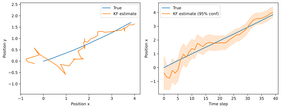
The left plot compares paths; the right shows the x position over time and the filter’s 95% confidence band.
Set conf=0.95 for a confidence ellipse with plot.estimate or plot.trajectory, or a confidence band with plot.signal.
Confidence visualization requires covariance data in the state or trajectory.
API quick reference
| Module | Main public interfaces |
|---|---|
sftools |
create_dynamics, create_observation, register_dynamics, register_observation |
sftools.types |
GaussianState, ParticleState, StateTrajectory |
sftools.model_dyn |
Linear, constant-velocity, and coordinated-turn models |
sftools.model_obs |
Linear, nonlinear, position, TOA, TDOA, and offset-range models |
sftools.estimator |
ls, wls, nls, NLSResult, KalmanFilter, UnscentedKalmanFilter, ParticleFilter |
sftools.helper |
ut, tt, mct, sigma_points, SigmaPoints, MCTResult, llh, crlb |
sftools.plot |
estimate, signal, trajectory |
For full signatures, consult the module docstrings in the source repository, which is available by invitation.
Example manual (PDF)
Download the example manual (PDF) for a more complete tutorial with worked examples, plots, and practice exercises on models, estimation, filtering, and moment transforms.